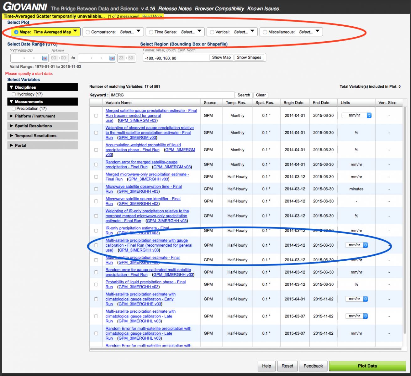
IMERG Early Run Example January 24th, 2020

Data Tutorials

STORM (https://storm.pps.eosdis.nasa.gov) is a publicly available Web-based data access interface for the Global Precipitation Measurement (GPM) Mission’s Precipitation Processing System (PPS). The goals of the 3D Visualization Pages are threefold. The first goal is to provide a way to visualize near real time data as soon as they become available on the ftp server. This is achieved through both the GPM Near Real Time Viewer and the STORM Event Viewer (EV)/EV Mini pages. The second is to allow users of the STORM data order interface to view products in three dimensions prior to order. For this, STORM Virtual Globe (VG) was created to complement the static images and Tool for High-Resolution Observation Review (THOR) Online tools. The final goal of these pages is to bring attention both to the work of the PPS group and the breadth of data coming from the GPM Core satellite and partner satellites processed by PPS. 

The STORM Virtual Globe web application allows you to view GPM data from STORM in an interactive 3D globe powered by Cesium.js. This tutorial will show you how to visualize GPM Dual-frequency Precipitation Radar data in 3D. 

Read the full STORM Virtual Globe user guide

  1. To gain access you must first register your email address at: https://registration.pps.eosdis.nasa.gov/registration/

  2. Once you have confirmed your registration, visit the STORM order website and enter the email address you used to register (in all lowercase): https://storm.pps.eosdis.nasa.gov/storm/data/Service.jsp?serviceName=Order
    STORM login screen

  3. When a valid email address has been entered, the rest of the interface will load onto the screen. You may then select your options for the data order. For the purposes of this tutorial, you can leave "Order Type", "Coincidence" and "Options" at their default values. 

  4. In the "Product Type" section, click the checkbox next to the "2ADPR" algorithm. This is the Level 2A processing of GPM Dual-frequency Precipitation Radar data, which provides 3D measurements of the precipitation within the atmospheric column. Learn more about the DPR here.
    STORM DPR selection

  5. The STORM Virtual Globe tool is also available for the following products: 2A GPROF, 2B CMB, 3A GPROF, IMERG Final Run Half Hourly 

  6. In the "Temporal Criteria" section, select the date range for the preciptiation data you would like to view. You may also select a specific geographic region in the "Options" section. 

  7. Once a valid date range has been selected, a list of GPM data products that match your criteria will be displayed in the "Search results" box. Each entry represents a GPM orbital swath that covers the period listed in the "Start Time" and "End Time" columns. 
    STORM swath selection

  8. Click the small globe icon  on the right side of the "Download / View" column to open this swath data in STORM Virtual Globe.

  9. Use the time slider control in the upper left of the interface to select the period of the swath you would like to view. The path of the GPM satellite and the current GMI swath being viewed is indicated by the white lines on the globe, while the DPR swath is within the red lines. 3D data is only available within the red DPR swath, and can only be seen when you zoom in close to the data. 

  10. Use the mouse to control the camera - the scroll wheel zooms in and out, clicking and dragging moves around the globe, and holding control while clicking and dragging will change the camera angle. Hovering over a data point will display its value in the info box. Click the "?" icon in the upper right of the interface for more details. The below screenshot shows GPM 2A DPR data from an overpass of Hurricane Irma on 9/5/17.
    STORM Virtual Globe interface

1. Search and select an interested variable

  • Go to the Giovanni website using the web browser of your choice: http://giovanni.gsfc.nasa.gov.
  • Type IMERG in the Keyword field and press the Search button. The resulting webpage should look like Figure 1 below.

The GIOVANNI webpage seen while searching for IMERG
Figure 1. The GIOVANNI webpage seen while searching for IMERG

There are currently 17 IMERG variables that will show up when you search. The various datasets all have a horizontal resolution of 0.1° x 0.1° and temporal resolutions of either 30 minutes or 1 month. Click here for a table with user-friendly descriptions of all the variables.

  • We will use the variable labeled “Multi-satellite precipitation estimate with gauge calibration – Final Run (recommended for general use)” as the focus of this tutorial. The blue oval in Figure 1 indicates this dataset for reference.
    • You can also plot monthly averaged data by choosing the 1st variable in the list above.
    • You can sort any of the parameters in the columns displayed above by clicking the column name.
  • Select the checkbox next to the variable of interest. This will automatically cause Giovanni to set boundaries for the Date Range so that you cannot select times without data.

2. Select plot type

Choose the type of plot you'd like to make. This tutorial will focus on making a standard “Time Averaged Map” that is selected by default. There is a red oval in Figure 1 around the menus that are used to select a type of plot.

3. Select temporal and spatial range

  • Choose the date range for the time averaged map. You can either type the date in or click on the small calendar icon next to the dates. For this tutorial we will choose August 1, 2014 at 00:00 UTC – August 2, 2014 at 23:59 UTC to plot the average of two days of data. Your date range should look like Figure 2 below.
     

Figure 2. The date range used for this tutorial.

Figure 2. The date range used for this tutorial.

  • Select the region over which you'd like to plot the data. IMERG data are currently available between 60°S – 60°N so Giovanni will not plot data beyond those bounds regardless of what is selected.
  • You can choose to only plot the data over a specific geographic region by either manually entering the latitude and longitude boundaries or by clicking the Show Map or Show Shapes button. For
  • This tutorial we will choose to plot the data over the United States shapefile.
  • Click on the Show Shapes button. Then click on Countries. Scroll down and click on the United States selection and then click the Done button in the lower-left corner of the shapes window. This is shown in Figure 3.

Figure 3. The shape selection window.

Figure 3. The shape selection window.

4. Make Plot

  • Now it's time to plot the data. Simply click the green Plot Data button in the lower right-hand corner of the page. 

You'll notice that precipitation over the United States is only plotted to 60°N. You can pan and zoom the map using the arrows and the + and – buttons in the upper-left corner of the map (or the mouse and mouse wheel). Figure 4 shows the resulting map focused over the continental United States.

Figure 4. The resulting map showing IMERG data focused on the continental United States.

Figure 4. The resulting map showing IMERG data focused on the continental United States.

5.  Download image or data

  • You can now either view the map within Giovanni or download the map in GeoTIFF or PNG format by pressing the Image button in the upper right hand corner of the image (circled in red in Figure 4).
  • You can also download a netCDF file containing the data plotted in the figure. To do this, click on the Downloads link on the right-hand side of the page under the History heading. You will see a link to download the netCDF file on the following page.

Discussion: 

For more information on GPM data at the GES DISC, see: http://disc.sci.gsfc.nasa.gov/gpm

To view a list of all of the GPM data holdings at GES DISC, see: http://disc.sci.gsfc.nasa.gov/uui/#/search/IMERG

Color Scale Range

Giovanni automatically chooses a color scale appropriate for the image based on the minimum and maximum values of the data being plotted. You can see that for this image Giovanni automatically chose the range of 0 mm/hr – 2.988 mm/hr.

To change this click on the Options button next to the Image button that is circled in Figure 4. In the window that pops up called Map Options you can change the minimum and maximum values.

Change Color Palette

The default blue to red color palette might not be appropriate for all users. To change this, click on the Options button next to the Image button that is circled in Figure 4. In the window that pops up called Map Options you can change the palette.

Change Data Smoothing

The data smoothing option, in the same Map Options window described above, allows you to apply GrADS' gxout shaded and bicubic smoothers to the data. Although this can be handy for low-resolution data, the effects on the 0.1° IMERG data are negligible.

Figure 5 below shows the resulting map created by setting the data range to 0 – 2 mm/hr, the color palette to White-Blue-Red-Yellow and the smoothing to On.

Figure 5. Map of IMERG data that uses all three optional tweaks.

Figure 5. Map of IMERG data that uses all three optional tweaks.

Overview:
The following instructions explain how to read the Version 6 IMERG HDF5 data product using the Python programming language.  Version 7 of this data product is read in the same way except that the precipitation variable in the half-hour product is called "precipitation" rather than "precipitationCal".  Both the half-hour and monthly IMERG files can be read using these instructions. For more information about the IMERG HDF5 data product, see the file specification and algorithm documentation available at the following URLS:

Instructions:
1. Install Anaconda Python 3, which includes the numpy, h5py, and matplotlib Python libraries.

2. Optionally, for displaying continent outlines, the following instructions will use the pyshp Python library, which can be added to an Anaconda installation using "conda install -c conda-forge pyshp". If following this procedure, then download a low-resolution global continent-outline shapefile for used when displaying the global data read from the IMERG HD5 file. One such shapefile is the coastline from Natural Earth: https://www.naturalearthdata.com/downloads/110m-physical-vectors/. The shapefile download file is called "ne_110m_coastline.zip".

3. Download an IMERG HDF5 file that covers either a full month or a half-hour period.  One source for IMERG HDF5 files is the GES DISC:

  • In a web browser, go to: http://mirador.gsfc.nasa.gov.
  • In the Keyword field, enter IMERG and press Search GES-DISC.
  • The first result shows monthly precipitation estimates, GPM Level 3 IMERG Monthly 0.1 x 0.1 degree Precipitation (GPM_3IMERGM). Click on View Files (see red arrow in Figure 1).
  • Click on the first file name in the list to download it. It is called, 3B-MO.MS.MRG.3IMERG.20150701-S000000-E235959.07.V03D.HDF5.

Alternatively, download an IMERG HDF5 file from the NASA Goddard Precipitation Processing System (PPS).  Before downloading data from PPS, register your email address at https://registration.pps.eosdis.nasa.gov/.  Then, visit the PPS online archive.  For example, to download the January 1, 2021, Final IMERG HDF5 files visit this URL: https://arthurhouhttps.pps.eosdis.nasa.gov/gpmdata/2021/01/01/imerg/.

4. Start an interactive session of Anaconda Python 3 by typing "python" on the command line of a Linux or MacOS system or by using the Start menu on a Microsoft Windows system.

5. Run the following python commands to read and display IMERG HDF5 data.

# -- read an IMERG HDF5 file
import numpy as np
import h5py
file='3B-HHR.MS.MRG.3IMERG.20210519-S000000-E002959.0000.V06B.HDF5'
data = h5py.File(file,'r')

# -- extract the 3600x1800 element precipitation array.
# For Version 6 IMERG HDF5 files, read the "precipitationCal"
# variable if it is a half-hour file and the "precipitation"
# variable if it is a monthly file.  For Version 7, the variable
# is "precipitation" for both durations.
precip = data['/Grid/precipitationCal'][:]

# -- get rid of the dummy single-element first dimension,
# transpose to get longitude on the x axis, and flip vertically
# so that latitude is displayed south to north as it should be
precip = np.flip( precip[0,:,:].transpose(), axis=0 )

# -- display the precipitation data. Regions with missing data
# values have negative values in the precip variable so allow
# the color table to extend to negative values.
import matplotlib.pyplot as plt
plt.imshow( precip, vmin=-1, vmax=10, extent=[-180,180,-90,90] )

# -- add a color bar
cbar = plt.colorbar( )
cbar.set_label('millimeters/hour')

# -- display lat/lon grid lines
for lon in np.arange(-90,90+1,90):
  dummy = plt.plot( (lon,lon), (-90,+90), color="black", linewidth=1 )

for lat in np.arange(-60,60+1,30):
  dummy = plt.plot( (-180,+180), (lat,lat), color="black", linewidth=1 )

# -- display the optional coastline shapefile
import shapefile as shp
shapeID = shp.Reader( 'ne_110m_coastline.shp')
for shape in shapeID.shapeRecords():
  point = np.array( shape.shape.points )
  dummy = plt.plot( point[:,0] , point[:,1], color="white",
    linewidth=1 )

# -- save the image to disk and display on the screen
plt.savefig('imerg.png',dpi=200)
plt.show()

# -- end of Python script

Credit: Tutorial updated by owen.kelley@nasa.gov in 2022.


Overview

Orbit Viewer THOR is a tool for displaying the satellite data files in the archive of the Global Precipitation Measurement (GPM) mission and Tropical Rainfall Measuring Mission (TRMM). THOR stands for “Tool for High-resolution Observation Review”. It is a point-and-click program written in IDL that  runs on Linux, Mac OS X, and Windows. This viewer enables you to display on a map of the Earth TRMM observations at the full instrument resolution.  Even if you plan on reading and analyzing GPM HDF5 files using your own IDL programs, it can help to have the THOR data viewer installed to do quick checks on the HDF5 files you are analyzing.

Full THOR Install Documentation: https://arthurhou.pps.eosdis.nasa.gov/thorrelease.html

Instructions

  1. Download the THOR data viewer .zip file from PPS: https://gpmweb2https.pps.eosdis.nasa.gov/pub/THOR/

    .
  2. Download the version that is most appropriate for your system. Once the zip file is downloaded, unzip it, and run one of the following scripts to install:

    1. MacOS: setupMAC.command

    2. Linux: setupUNIX.sh

    3. Microsoft Windows: setupWIN.bat

  3. Once the setup script has finished, run the new executable file that was created to launch THOR. Full documentation for using THOR is located in the unzipped THOR install directory under Doc > Tutorial.pdf.

  4. In order to download data from the GPM online archive you must first register your email address with the Precipitation Processing System (PPS), using this page: https://registration.pps.eosdis.nasa.gov/

  5. Download your desired HDF5 data files from the online archive: https://arthurhouhttps.pps.eosdis.nasa.gov/ . When prompted, use the email address that you just registered with PPS as both the username and password for logging into the online archive.

    1. The structure of directories indicates the type of data you will be accessing. For example, going to https://arthurhouhttps.pps.eosdis.nasa.gov/gpmdata/2021/01/01/gprof Will lead you to precipitation estimates for passive microwave instruments calculated by the GPROF algorithm for January 1, 2021.

    2. The HDF5 file name provides information about the data in the file. For example, the filename 2A-CLIM.GPM.GMI.GPROF2021v1.20210101-S013133-E030407.038882.V07A.HDF5 indicates that the algorithm is the GPROF algorithm, the start datetime is January 1, 2021, at 0131 UTC, the end time is 0304 UTC, the GPM orbit number is 38,882, and the data version is 7A.

  6. Use the THOR program to open the file using File > Open File menu option.

  7. You can navigate the structure of the HDF5 file using the left side of the THOR main window. The right side of the THOR main window displays your selected info, depending on what kind of data you are viewing. Each algorithm contains. The file formats are described on the "PPS/GPM Documentation" page of the PPS website and the algorithms that create them are described on the "Algorithm Theoretical Basis Documents" page of the PPS website (https://arthurhou.pps.eosdis.nasa.gov/).

  8. Here is an example. To view the precipitation rate in a Final IMERG half-hour HDF5 file, double click on "Grid" and then click on "precipitationCal". In the global view, click on the Gulf of Mexico to see a zoom image of the precipitation in that region.

    Image

Credit: Tutorial updated by owen.kelley@nasa.gov in 2022.

Overview: 

Satellite observation and climate model data become more and more widely used in GIS.  ArcGIS is one of the dominant software packages in the GIS community. NetCDF format is not a traditionally used GIS format although it is getting popular in the community.  This recipe shows how to import a grided model or satellite (Level 3 or Level 4) data file in NetCDF format into ArcGIS. 

Best When: 

The data is in CF-complaint NetCDF format 

Task: 
Viewing Data
 
Example: 
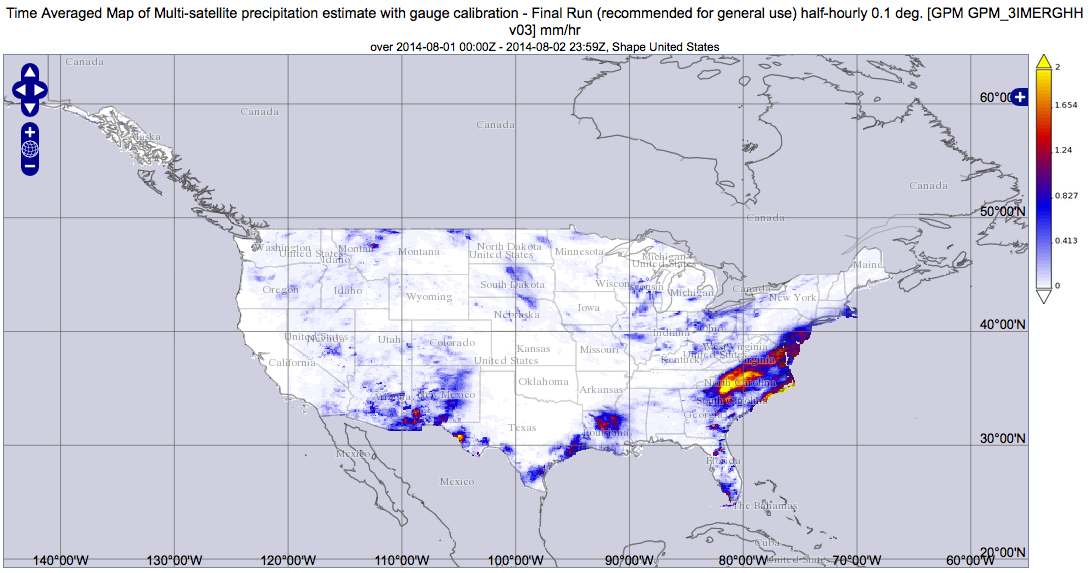
Import a TRMM monthly  precipitation data file into ArcGIS.
 
Estimated time to complete the folllowing procedure: 5 min
 

Procedure: 

1) Getting data in NetCDF format

The original data format of TRMM products is HDF.  There are a number ways to obtain the data in CF-compliant NetCDF format from GES DISC.  In this example, the monthly data (Sep 2012) was downloaded from OPeNDAP service at:

https://disc2.gesdisc.eosdis.nasa.gov/opendap/TRMM_L3/TRMM_3B43.7/2012/3B43.20120601.7.HDF.html
 
Clicking on “Get as NetCDF” button to download the file:
nc_3B43.20120901.7.HDF.ncml.nc

2) Import data into ArcGIS
  • Start an ArcGIS Application, for example, ArcMap

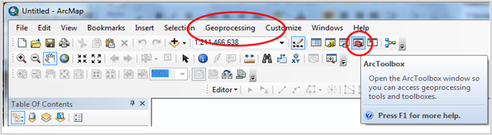
  • Open the ArcToolbox window with the Show/Hide ArcToolbox Window button  found on the standard toolbar or by clicking Geoprocessing -> ArcToolbox (Figure 1)

ARCGis Example screenshot

Figure 1: Sample of ArcMap start page

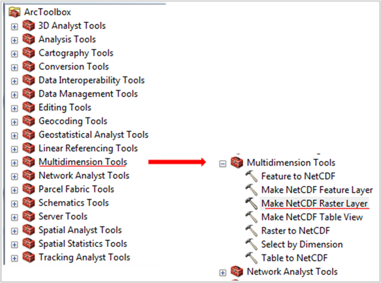
  • From ArcToolbox --> Multidimensional Toolbox --> Make NetCDF Raster Layer (Figure 2)

ARCGis Example screenshot

Figure 2: Sample of ArcToolbox of ArcMap

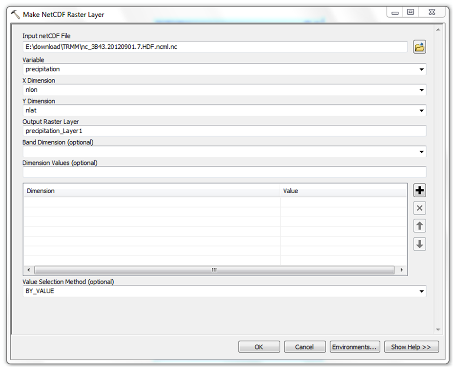
  • Select the input file, the variable to be imported, and the X and Y dimensions of the data.  In this example, the variable to be imported is “precipitation” and the X dimension is “nlon” and the Y dimension is “nlat” (Figure 3).  The X and Y dimensions are the coordinate variables included in the NetCDF file and they are usually very easy to be identified from the pull down menu, e.g., often being named something like “longitude” and “latitude”

  • You may modify the Output Raster Layer name, default is "precipitation_Layer 1"

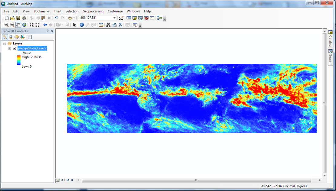
  • Click “Ok”  at the bottom to add the variable and an image will be displayed as in Figure 4

ARCGis Example screenshot

Figure 3: Sample of Make NetCDF Raster Layer in ArcMap


ARCGis Example screenshot

Figure 4: Sample TRMM Level 3 monthly precipitation displayed in ArcMap


Discussion: 

CF-compliant NetCDF data will be imported with georeferencing information being correctly carried over.  For none CF-compliant NetCDF data, georeferencing information may be not exist or not be imported correctly.  It is important to correctly identify the dimension in the data file.
 
The ArcGIS “Make netCDF Raster Layer” tool requires that the data have equal spacing along each dimension.  Thus, satellite swath data (Level 1 or Level 2) cannot be imported using above method, in which case the “Make netCDF Feature Layer” can be used.  See the recipe "How to Import Swath Data in NetCDF format into ArcGIS" for more information.
 
Some satellite data contains vertical and/or time dimension.  These dimensions can be defined in ArcGIS. See the recipe "How to Define Vertical and Temporal Dimensions in ArcGIS" for more information

Hide Date