
Yes, in line with NASA's general data policy. Please refer to the GPM Data Policy for further details.
Frequently Asked Questions
Data
For questions about permission for using NASA images and videos, please refer to NASA's official Media Usage Guidelines. For any additional questions please contact bert.ulrich@nasa.gov
There are several sources for downloading and viewing data which allow you to subset the data to only include specific parameters and/or geographic locations. These include the GES DISC, Giovanni and STORM. In Giovanni you can obtain data for a specific country, U.S. state, or watershed by using the "Show Shapes" option in the "Select Region" pane.
There are several sources for downloading and viewing data which allow you to subset the data to only include specific parameters and/or geographic locations. These include the GES DISC, Giovanni and STORM. In Giovanni you can obtain data for a specific country, U.S. state, or watershed by using the "Show Shapes" option in the "Select Region" pane.
The TRMM satellilte has been decommissioned and stopped collecting data in April 2015. The transition from the Tropical Rainfall Measuring Mission (TRMM) data products to the Global Precipitation Measurement (GPM) mission products has completed as of August 2019. The GPM IMERG dataset now includes TRMM-era data from June 2000 to the present, and other TRMM-era data has been reprocessed with GPM-era algorithms and is now available on the GPM FTP servers. TMPA data production ended as of December 31st, 2019 and the TRMMOpen FTP server has been shut down. Historical TMPA data is still available to download from the NASA GES DISC at: https://disc.gsfc.nasa.gov/datasets?keywords=TMPA&page=1
Click here for more details on the transition from TMPA to IMERG.
GPM data products can be divided into two groups (near real-time and production) depending on how soon they are created after the satellite collects the observations. For applications such as weather, flood, and crop forecasting that need precipitation estimates as soon as possible, near real-time data products are most appropriate. GPM near real-time (GMI & DPR) products are generally available within a few hours of observation. For all other applications, production data products are generally the best data sets to use because additional or improved inputs are used to increase accuracy. These other inputs are only made available several days, or in some cases, several months, after the satellite observations are taken, and the production data sets are computed after all data have arrived, making possible a more careful analysis.
For the GPM IMERG dataset, IMERG Early and Late Runs are the near real-time products, while IMERG Final Run is the research / production product. Click here to learn more about the differences between IMERG Early, Late and Final.
The resolution of Level 0, 1, and 2 data is determined by the footprint size and observation interval of the sensors involved. Level 3 products are given a grid spacing that is driven by the typical footprint size of the input data sets.
For our popular multi-satellite GPM IMERG data products, the spatial resolution is 0.1° x 0.1° (or roughly 10km x 10km) with a 30 minute temporal resolution.
Visit the directory of GPM & TRMM data products for details on the resolution of each specific products.
Browse our directory of GPM & TRMM data products to locate your desired algorithm, then click on the links in the algorithm description under "Documentation". All documentation is also available at the Precipitation Processing System website.
Precipitation
Not really. Raindrops start out as round cloud droplets. As they grow and start falling, they begin to experience the resistance of the air, which causes them to flatten and resemble tiny M&M candy. Further growth leads to thinning in the center of the M&M, until the eventual breakup of the drop.
The flattening of raindrops alters the echo they produce when "illuminated" by radar from the side. But for a space-borne radar such as the GPM DPR, the effect is minimal.
Watch the below video to learn more:
This short video explains how a raindrop falls through the atmosphere and why a more accurate look at raindrops can improve estimates of global precipitation.
This video is public domain and can be downloaded at: http://svs.gsfc.nasa.gov/goto?11288
Drops vary in size from the tiny cloud droplets (measuring less than 0.1 mm in diameter) to the large drops associated with heavy rainfall, and reaching up to 6 mm in diameter. Collision among drops and surface instabilities are generally thought to impose this 6-mm size limit, although drops as large as 8 mm in diameter have been reported in shallow warm showers in Hawaii.
The reflectivity of a drop when illuminated by radar is roughly proportional to the square of its volume. It is this property which radar meteorologists exploit to estimate the total volume of rain from the reflectivity observed. This estimation process is rather difficult because the radar-rain relation is not linear, and the range of drop sizes within a single storm can vary greatly.
Hail stones vary in size. Most commonly they are 1 cm in diameter but have been observed to be as large as 10 to 15 cm. Hailstones are formed when either aggregated ice ("graupel") or large frozen raindrops grow by collecting cloud droplets with below-freezing temperatures. An important aspect of hail growth is the latent heat of fusion which is released when the collected cloud water freezes. So much liquid water is collected in the process of hail growth that the latent heat released can significantly affect the temperature of the hailstone and make it several degrees warmer than the cloud environment. As long as the temperature of the hailstone remains below 0° C, its surface remains dry and its development is called "dry growth". The heat transfer from the hailstone to the surrounding air, however, is generally too slow to keep up with the release of heat associated with the freezing of the collected cloud drops. Therefore, if a hailstone remains in a supercooled cloud long enough, its temperature can rise to 0° C. At this temperature the collected supercooled droplets no longer freeze immediately upon contact with the hailstone. Although some of the collected water may be lost to the warm hailstone by shedding, a considerable portion can remain to be incorporated into the stone forming a water-ice mesh that is called "spongy hail". This process is called "wet growth". During its lifetime, a hailstone may grow alternately by the dry and wet processes as it passes through air of varying temperature. When hailstones are sliced open, they often exhibit a layered structure, which is evidence of these alternating growth modes. Hailstones need time to grow before they become too heavy and fall to the ground. An empirical relation between the fall velocity of a hailstone and its diameter is given by
V = 9 exp(0.8ln(D)) m/s,
where D is the diameter in cm. Hence a hailstone with a diameter on the order of 15 cm will fall at 75-80 m/s (170-180 miles/hour)!! This implies that updrafts of a comparable magnitude must exist in the cloud to support the hailstones long enough for them to grow. Because of this, hail is found only in very intense thunderstorms. Therefore, hail detection in storms is a clear indicator of their severity.
The GPM DPR has specific channels which can detect frozen particles in general and hail in particular. This helps provide crucial information about storm severity.
Hail forms when thunderstorm updrafts are strong enough to carry water droplets well above the freezing level. This freezing process forms a hailstone, which can grow as additional water freezes onto it. Eventually, the hailstone becomes too heavy for the updrafts to support it and it falls to the ground.
This question is tricky because some precipitating raindrops may not fall at all, if the surrounding wind has a sufficiently strong upward component. In still air, the terminal speed of a raindrop is an increasing function of the size of the drop, reaching a maximum of about 10 meters per second (20 knots) for the largest drops. To reach the ground from, say, 4000 meters up, such a raindrop will take at least 400 seconds, or about seven minutes.
The GPM DPR has the capability to measure the fall speed of precipitating particles, which is important because it helps characterize the type of rain being measured.
Rain rates up to 400 millimeters per hour have been measured in particularly strong tropical cyclones. However, even within the strongest storms, such high instantaneous rates are rarely sustained for periods longer than a minute, although a point on the ground can accumulate as much as 1800 millimeters per 24 hours during the passage of an exceptionally strong rainstorm.
This important question is still under investigation. Much of the rain is produced by clouds whose tops do not extend to temperatures colder than 0° C. The mechanism responsible for rain formation in these "warm" clouds is merging or "coalescence" among cloud droplets, which are first formed by vapor condensation. Coalescence is probably the dominant rain-forming mechanism in the tropics. It is also effective in some mid-latitude clouds whose tops may extend to subfreezing temperatures. However, once a cloud extends to altitudes where the temperature is colder than 0° C, ice crystals can form and "ice-phase" processes become important. In favorable conditions, ice-involving processes can initiate precipitation in half the amount of time water-only processes would need. Hence, at mid-latitudes, cumulus cloud rain is probably initiated by ice-processes and melting of ice. Observations have shown, however, that precipitation can first appear at levels warmer that 0° C, where vapor condensation and coalescence are the main rain producers. Thus, precipitation may be initiated by either process.
Depending on their type, clouds can consist of dry air mixed with liquid water drops, ice particles, or both. Low, shallow clouds are mostly made of water droplets of various sizes. Thin, upper level clouds (cirrus) are made of tiny ice particles. Deep thunderstorm clouds which can reach up to 20 km in height contain both liquid and ice in the form of cloud and raindrops, cloud ice, snow, graupel and hail.
It is important to understand that even a cloud that looks impenetrably dark is almost entirely made of dry air. Water vapor and precipitation each make up a maximum of just a couple of percent of the mass of a cloud, except in a few very intense storms.
How do these precipitation particles form? First, tiny cloud droplets are born when the water vapor in the air is cooled and starts to condense around tiny "condensation nuclei" (particles so small they are invisible to the naked eye). The presence of these aerosols is crucial: without them, in absolutely clean air, condensation would not start until the relative humidity has reached several hundred percent (this suggests that the "saturation" level of 100% humidity is poorly defined; in fact, the atmosphere always contains more than enough nuclei of all sorts for condensation to start as soon as the dew point temperature is reached). The more particles there are in the atmosphere, the easier cloud droplets will be formed and the smaller they will be (since more particles will be competing for the same amount of water, so each one of them will attract less). This is why clouds over land have more droplets of smaller sizes than clouds over oceans where the air is generally much cleaner.
The process of ice formation similarly requires the presence of nuclei. However, there are much fewer particles which make suitable ice nuclei. This is why freezing often does not start until the temperature of the air reaches -15° C (if there are no ice nuclei at all, freezing will not occur before the temperature drops to -40° C). Hence, clouds with temperatures below 0° C can still consist of water droplets called "supercooled" water. These drops freeze immediately upon contact with any surface. When they fall to the ground as freezing rain, they can form a thin layer of sleet on roadways, an almost invisible and very dangerous hazard for drivers.
Precipitation forms when cloud droplets or ice particles in clouds grow and combine to become so large that the updrafts (e.g. upward moving air) in the clouds can no longer support them, and they fall to the ground.
Availability of water vapor and intensity of updrafts within a cloud determine the size of a raindrop. Larger drops tend to result from the vigorous updrafts within a thunderstorm and fall faster than smaller drops. Mist or drizzle produce smaller drops that fall at lower speeds.
Wind flow up a mountain tends to enhance precipitation – when the air moves higher into the atmosphere it is cooled, which drops the saturation dew point, and therefore tends to make more moisture available. Wind blowing down the mountain does the opposite. If the atmosphere is sufficiently unstable, the lift provokes deep convection. But in less convective situations, the extra moisture is squeezed out in the lowest layers of the atmosphere, mostly as the entirely liquid “warm rain process”. Either way, orographic (mountainous) effects create fine-scale variability that challenges all observations:
- More rain gauges are needed to pick up the variability, but there are almost always fewer gauges in the mountains.
- Surface radars can’t see all the way to the surface due to blockage of the radar beam, ground clutter, and the increasing height of the lowest beam with height.
- Satellite radars can’t see all the way to the surface due to ground clutter.
- Satellite passive microwave radiometers over land depend on channels that sense frozen hydrometeors (snow, graupel, hail), but in countries such as Puerto Rico, these frozen hydrometeors are only present at altitudes of 4 or more kilometers above the surface. So, if the orographic enhancement is in deep convection, then the satellite signal is relatively well-correlated to surface rain. But when the extra boost is due to warm rain enhancement, the satellite signal might only have a weak relation to the surface rainfall.
- Satellite infrared sensors only see the cloud tops, and as for the passive microwave sensors, warm rain processes near the surface can be more or less decoupled from what’s happening in the upper reaches of the cloud.
- Various numerical model-based estimates have issues, which include the time/space scale of the computation being too coarse to adequately resolve the processes, approximations in the microphysics (conversions among vapor, droplets, and ice particles) that are not sufficiently accurate, and shortcomings in the input observations needed to feed the computation the correct upstream conditions.
Because of these factors, satellite based estimates of precipitation in mountainous regions may be less accurate than ones in non-mountainous regions. For the IMERG product, you can get an idea of the accuracy of a given precipitation estimate by checking the quality index. Learn more.
Usually up to the "freezing level", where the temperature has decreased to below 0° C (over the tropics, that occurs at about 5000 meters; over Los Angeles, it fluctuates between 2000 and 4000 meters in winter, and between 4000 and 5000 meters in summer). In different types of rain, there can be frozen water such as hail mixed with the rain below the freezing level, and/or "super-cooled" liquid drops above it.
In most storms, the GPM DPR is very good at detecting the freezing level. The GPM DPR has separate channels to identify frozen, melting, and liquid particles, thereby providing very detailed information about the evaporative cooling and/or condensational heating released into the atmosphere by rainstorms.
IMERG
The most frequent number of samples of PMW data for an IMERG grid box in any given 30-minute period is overwhelmingly zero, with one in most of the rest. In a very few cases there are two or more. However, the histogram of single values of precipitation rate differs substantially from histograms of two, three, or four averaged together. Once the team realized this several IMERG versions ago, they instituted a down-select scheme to provide the single "best" PMW estimate in each grid box at each time. The GEO-IR brightness temperatures used are from the Climate Prediction Center (CPC) Merged 4-km Global IR data product, which gives the "best" GEO-IR value each half hour in each ~4x4 km (at the Equator) grid box. The down-select of GEO-IR to a consistent number of samples (here, one) in a half hour is done at the CPC, which ensures that the GEO-IR values are all drawn from nearly the most consistent record achievable. Inter-satellite differences and differences in retrievals due to surface climate regime are still realities for both PMW and GEO-IR.
To summarize, there are multiple values for both PMW (occasionally) and GEO-IR (with a frequency depending on the satellite being used at any given time and place), but:
- Organized records of the not-selected passive microwave samples do not exist - although a user could construct this from the PPS archive of all the Level 2 products.
- Accessing “all” the GEO-IR is a daunting task - and these data would be brightness temperatures, not precipitation estimates.
As such, IMERG is best described as "half-hourly snapshots". The IMERG team suggests that the most sensible way to use these data is to treat them as the average for the half-hour period, since there is no additional information about the sub-half-hourly sequence of events, particularly in the case where the IMERG value is based on "morphed" passive microwave values from other times.
Both TMPA and IMERG use a constellation of passive microwave satellites, and within the general umbrella groups of “sounder” and “imager” the inputs are much the same, although at the end of the TRMM era the TMPA was not upgraded to include the newer satellites. The direct inputs of the TMI and GMI are swamped by the amount of data from the rest of the microwave sensors, so the absence of TMI in the last 4.5 years of TMPA was not a major problem. At the back end of the multi-satellite algorithms, both TMPA and IMERG use the same scheme for combining satellite data with the GPCC analysis, although IMERG uses the GPCC Final analysis up through 2018, which tends to be more accurate than the GPCC Monitoring analysis that the TMPA used for the last ~9 years. What’s different? The algorithms for the Combined products are very different (2B31 for TMPA and CORRA for IMERG), and that is what provides calibration. The GPROF algorithm has been upgraded for use in IMERG – still Bayesian, but with the libraries of profiles sourced and organized differently. The IR scheme has shifted from VAR to PERSIANN-CCS – very different approaches. Compared to the simple chunking of data into 3-hour intervals in TMPA, note the massive amount of time spent in IMERG on morphing and the Kalman filter. The goal is two-fold:
- Provide a finer time resolution so that system evolution is more accurately captured, compared to the 3-hour interval in TMPA. This improved evolution not only provides morefrequent data values, but it should also make the IMERG time averages (such as daily) more accurate, since precipitation changes so rapidly in space and time.
- Reduce the use of IR estimates, which have low quality, by time-interpolating the microwave estimates, which have better quality. The hard part here is that the interpolation has to be done in a quasi-Lagrangian framework because the rain systems move. So, IMERG’s morphing/Kalman framework is intended to minimize the IR contribution, even though IR is still seen as necessary in regions with long microwave gaps.
Please view the document The Transition in Multi-Satellite Products from TRMM to GPM (TMPA to IMERG) for further details.
IMERG provides a data field that estimates the probability that the retrieved precipitation amount is “liquid”, which is defined to include “mixed” (liquid and solid) precipitation. In retrospect the field name should have been “ice”, but “liquid” had already been set. The rational is that mixed precipitation is very rare and transient, so it should be lumped with either “liquid” or “ice”. Furthermore, the primary effects of “ice” are to 1) prevent the falling precipitation from immediately entering the hydrological system (until it melts), and 2) to create (potentially) dangerous travel conditions. “Mixed” typically ends up not creating either of these effects, so lumping it with “liquid” seems appropriate.
Even given this basic definition, there are numerous forms of precipitation, and it might not be obvious how they end up being classified in IMERG. The key fact is that the phase is computed diagnostically at present, based on work by Guosheng Liu (Florida State University) and students. The Liu scheme uses data from a numerical model or model analysis to compute a “specification”, without reference to the satellite data, including whether or not IMERG estimates that precipitation is occurring, or even possible to estimate. Thus, probabilityLiquidPrecipitation (pLP) is a globally complete field whenever the relevant model data exist. An additional factor is that there is a conceptual difference between how the half-hourly phase is computed and how phase is defined in this probability framework for the monthly data. We will handle the half-hourly first, for which the Liu specification equation is directly relevant.
Liu determined that the primary factor for phase is the surface wet bulb temperature (Tw), a combination of temperature and humidity, with small contributions from the low-altitude Tw lapse rate and the surface pressure, and with systematic differences between ocean and land areas. In practice, the fitted probability as a function of Tw is converted to separate look-up tables for ocean and land.
Typical results for different forms of precipitation are:
- Rain: Ordinary falling liquid typically happens for Tw>0°C, so pLP is high.
- Freezing Rain: Liquid that freezes upon contact with the Earth's surface typically falls in Tw<0°C, so pLP is low.
- Snow, ice pellets, snow pellets: These frozen hydrometeors occur around or below Tw<0°C, so pLP varies from around 50% to very low.
- Sleet: Frozen droplets (U.S. definition) typically fall in Tw<0°C, so pLP is usually below 50%.
- Mixed snow and rain; falling slush: The mixed category is likely to occur around the pLP=50% mark. If one uses 50% as a liquid/solid threshold, that implies that mixed cases will end up in both categories, depending on the details.
- Hail: Hail typically occurs when the surface air temperature is well above freezing (i.e., on summer afternoons). Thus, pLP is very high. But, hail is even rarer than mixed and unlikely to be correctly specified in this scheme, and anyway, in such conditions it rapidly melts and so is properly lumped into "liquid".
- Dew and frost: These phenomena are not forms of precipitation. They are liquid or solid water that condenses directly at the Earth's surface. For this reason, any amount of surface accumulation due to dew or frost is not included in the IMERG precip estimate.
As the time interval for the data values lengthens, it becomes increasingly likely that both liquid and solid might have fallen, at which point the meaning of pLP should change to “what fraction of the estimated precipitation amount fell as liquid or mixed?” This is the definition of pLP for both the monthly IMERG Final Run pLP and the set of GIS IMERG files (TIFF+WorldFile) providing estimated accumulations longer than three hours.
Q1: How closely should the monthly satellite-gauge combined precipitation datasets follow the gauge analysis?
A1: The combined precipitation research team at Goddard has major responsibility for the Global Precipitation Climatology Project monthly Satellite-Gauge combined product, the Tropical Rainfall Measuring Mission (TRMM) Multi-satellite Precipitation Analysis (TMPA) 3B43 monthly product (previously), and the IMERG Final Run monthly product. In each case the multi-satellite data within the product are averaged to the monthly scale and combined with the Global Precipitation Climatology Centre's (GPCC) monthly surface precipitation gauge analysis (see https://www.dwd.de/EN/ourservices/gpcc/gpcc.html). In each case the multi-satellite data are adjusted to the large-area mean of the gauge analysis, where available (mostly over land), and then combined with the gauge analysis using a simple inverse estimated-random-error variance weighting. In all three data sets the gauge analysis has an important or dominant role in determining the final combined value for grid boxes in areas with "good" gauge coverage. Regions with poor gauge coverage, such as central Africa have a higher weight on the satellite input. The oceans are mostly devoid of gauges and therefore mostly lack such gauge input. Isolated island stations are deleted from the GPCC gauge analysis before use because they are usually not representative of the surrounding ocean, and frequently not even the island as a whole.
Q2: How closely related are the short-interval multi-satellite precipitation datasets to the monthly satellite-gauge combined precipitation datasets?
A2: The short-interval GPCP is the One-Degree Daily (1DD), the short-interval TMPA is 3B42 (which is 3-hourly), and the short-interval IMERG is the half-hourly. In each case the short-interval data are adjusted with a simple, spatially varying ratio to force the multi-satellite estimates to approximately average up to the corresponding monthly product, although with controls on the ratios to prevent unphysical results. Thus, monthly-average values for the short-interval data should be close to the mean values for the monthly datasets, which the developers consider more reliable than the short-interval datasets. In fact, compared to datasets that lack the adjustment to the monthly satellite-gauge estimates, the 1DD, 3B42, and IMERG Final half-hourly datasets tend to score better at timescales longer than a few days. This is presumably because the random error begins to cancel out as more samples are averaged together, while the bias error remains.
As an example, see:
Bolvin, D.T., R.F. Adler, G.J. Huffman, E.J. Nelkin, J.P. Poutiainen, 2009: Comparison of GPCP Monthly and Daily Precipitation Estimates with High-Latitude Gauge Observations. J. Appl. Meteor. Climatol., 48(9), 1843–1857.
In the previous TMPA data set, each data value provided a precipitation rate based on one (or perhaps two) satellite snapshots during the TMPA’s 3-hour analysis period. IMERG values are based on a single microwave snapshot during its half-hour analysis period, or a morphed/Kalman filter interpolation if no microwave values are available. The values are expressed in the intensive units mm/hr; it is usually best to assume that this rate applies for the entire half-hour period. If you wish to regrid to a finer time and/or space grid, note that many interpolation schemes have the property of suppressing maxima in precipitation and expanding rain events into neighboring zero-amount periods, so it is critical that you examine this issue and state what scheme was used in documentation and papers.
The entire record for each Run (Early, Late, or Final) is computed with the same version of processing, with the same input steams specified for that Run. The data that are processed afresh are called “Initial Processing” (IP) and those that processed after the fact when the new version starts are called “retrospective processing” (RP). The RP have a couple of simplifications that the team doesn’t believe are important, but should be mentioned for completeness:
- The precipitation from the individual satellites is computed with the GPROF algorithm using a different source of temperature and humidity ancillary data. In the aggregate, the results are very similar.
- The entire set of input data is used in RP, whereas in IP it is possible that some of the input will have been delayed and there are not available to create the IP products. The latency for computing the Early, in particular, is set to wait long enough that we usually capture 85-90% of the eventual input.
A final point is that the complement of satellites and (sometimes) their overpass times change over time. To the extent that different sensors “see” different interpretations of the precipitation, and the IMERG intercalibration is not entirely able to overcome this, the team expects at least slight variations over time in quality and performance. This issue is less critical if you are looking at mean behavior, but more important if you are trying to estimate extremes.
The main difference between the IMERG Early and Late Run is that Early only has forward propagation (which basically amounts to extrapolation forward in time), while the Late has both forward and backward propagation (allowing interpolation). As well, the additional 10 hours of latency allows lagging data transmissions to make it into the Late run, even if they were not available for the Early (see below).
There are two possible factors which contribute to differences in the IMERG Late Run and Final Run datasets:
- The Late Run uses a climatological adjustment that incorporates gauge data. In Versions 05 and 06 no adjustment has been applied. In Version 04 this was a climatological adjustment to the Final run, which includes gauge data at the monthly scale. For Version 03 the TRMM V7 climatological adjustment of the TMPA-RT to the production TMPA was used (which includes gauge at the monthly scale) because this at-launch algorithm didn't yet have any Late and Final data from which to build the climatological adjustment. The Final run uses a month-to-month adjustment to the monthly Final Run product, which combines the multi-satellite data for the month with GPCC gauge. Its influence in each half hour is a ratio multiplier that's fixed for the month, but spatially varying.
- The Late Run is computed about 14 hours after observation time, so sometimes a microwave overpass is not delivered in time for the Late Run, but subsequently comes in and can be used in the Final. This would affect both the half hour in which the overpass occurs, and (potentially) morphed values in nearby half hours.
The satellite sensor difference could be examined by comparing the satellite sensor data field in the Late and Final Run datasets for each half hour. Since the gauge adjustment is a constant multiplier, a time series should show a constant ratio between the Late and the Final Runs for the entire month (except for cases where the satellite sensor is changing, just as for the ocean).
We always advise people to use the Final Run for research. The vast majority of grid boxes have fairly similar Late and Final values, so it makes sense to stick to metrics that are more resistant to occasional data disturbances. Extreme values are more sensitive to these details; medians, means, and root-mean square difference are less sensitive.
The following table provides a quick reference for the IMERG variables that can be visualized using Giovanni.
|
Product |
Variable and Description |
|---|---|
|
GPM_3IMERGHHE 30-min averaged data |
Merged microwave-only precipitation estimate [Final] Precipitation estimates from combining microwave data from the GMI, TMI, and other partner instruments. |
|
Random error for gauge-calibrated multi-satellite precipitation [Final, Early, Late] This is an estimate of the non-systematic component of the error. The exact variable name depends on the product, but all begin with "Random error..." |
|
|
Microwave satellite observation time [Final] Observation time of the microwave precipitation estimates given as minutes from the beginning of the current half-hour. |
|
|
Microwave satellite source identifier [Final] This is an integer between 0 and 24 that corresponds to the instrument from which the microwave precipitation estimate was taken. See *3IMERGHH data fields* in the Integrated Multi-satellitE Retrievals for GPM (IMERG) Technical Documentation |
|
|
Weighting of IR-only precipitation relative to the morphed merged microwave-only precipitation estimate [Final] This is the weighting of the infrared data in the final merged estimate, given in percent. Zero means either no IR weighting or no precipitation. |
|
|
IR-only precipitation estimate [Final] This is the microwave-calibrated infrared precipitation estimate. |
|
|
Multi-satellite precipitation estimate with (climatological) gauge calibration [Final, Early, Late] This is the precipitation estimate that is calibrated with monthly gauge data for the Final Run. This variable is recommended for most users. Note: The gauge calibration used in Early and Late would be climatological, but in V06 no calibration is applied in either Early or Late. |
|
|
Multi-satellite precipitation estimate [Final] This is the precipitation estimate that has not been calibrated with gauge data. |
|
|
Accumulation-weighted probability of liquid precipitation phase [Final] This is the probability of liquid precipitation. The probabilities are calculated globally regardless of whether precipitation is actually present |
|
|
GPM_3IMERGM 1 month averaged data |
Weighting of observed gauge precipitation relative to the multi-satellite precipitation estimate This is the percent weighting of the surface gauge data. |
|
Merged satellite-gauge precipitation estimate This is the precipitation estimate that has been calibrated with gauge data. This variable is recommended for most users. |
|
|
Accumulation-weighted probability of liquid precipitation phase This is the probability of liquid precipitation. The probabilities are calculated globally regardless of whether precipitation is actually present. |
|
|
Random error for merged satellite-gauge precipitation This is an estimate of the non-systematic component of the error. |
1. Most of the low-orbit microwave satellites downlink their data once or twice an orbit (which is about 90 minutes long) to the operating agency. [Except GMI comes down in 5-min. granules.] The agencies compute the Level 1B files, package them, and ship the data around. PPS gets all the NOAA and EUMETSAT data through NOAA, DMSP from NRL Monterey, and the Japanese AMSR2 through NASA, SAPHIR (now intermittently and generally not in near-real time) through ISRO, and GPM DPR and GMI within GPM. The global merged geo-IR data are assembled by NOAA/NWS/CPC, and the Precipitation Processing System (PPS) accesses GEOS FP forecasts through the Goddard NCCS and Autosnow from NOAA. By about 3 hours after observation time the geo-IR and about 85% of the microwave (depending on how systems feel that day) have arrived at PPS. PPS converts the microwave data to precip estimates and computes the IMERG Early Run, which only uses forward propagation morphing (plus IR in the Kalman filter) by about 4 hours after observation time. [One subtle point is that the IR half-hour data fields come in pairs, so both halves of the hour are processed together, meaning the second half hour almost always has shorter latency than the first. Another is that IMERG uses forecasts to get the analysis of vertically integrated vapor, which is what IMERG V06 uses to estimate system motion for the morphing. So, hitches in delivery of the latest GEOS FP are not a big deal – IMERG just uses the most recent forecast sequence, whatever that is.]
2. To compute the IMERG Late Run, which entails both forward and backward propagation morphing (plus IR), processing has to wait long enough that the following microwave overpass has a chance to occur and then follow the delivery chain described above. So, PPS waits 11 hours to capture a reasonably complete set of "next overpass" data, and then start processing. The nominal latency stated in the documentation is 14 hours, but it's more like 12 in recent data.
3. The IMERG Final Run uses MERRA2 for the vertically integrated vapor, GPCC monthly Monitoring Analysis for gauge, and revised precipitation retrievals that depend on ERA-5 (and ERA-I up through mid-2019). The pacing items are the GPCC and ERA-5, usually giving a latency of about 3.5 months.
Compared to previous versions, Version 06 IMERG introduces additional coverage at the high latitudes for the precipitation fields in all Runs -- Early, Late, and Final. IMERG continues to use a merged geosynchronous infrared brightness temperature analysis to provide IR-based precipitation estimates. The requisite analysis (provided by NOAA/NWS/Climate Prediction Center) covers the latitude band 60°N-S, so a "full" IMERG analysis is possible there. At higher latitudes (in both hemispheres) IR-based estimates cannot be included, so the coverage in the complete precipitation fields is "partial" -- limited to gridboxes for which there is no snow/ice on the surface. Some of the other data fields, specifically the merged microwave estimates and the precipitation phase, are provided for the entire globe.
Climate, hazards, and the water cycle
Weather satellites have been used by the National Weather Service since the sixties to map clouds, sea surface temperatures, and vertical temperature and moisture distributions. These data are supplemented by crucial ground observations, and are subsequently input to numerical models which try to predict the short-term evolution of the weather. The results are then made available to the public, most directly in the form of composite weather maps. The rain shown on these maps comes mostly from ground weather radars.
Unfortunately, the crucial ground observations are often simply not available because these regions are typically inaccessible. In addition, the large-scale numerical models are still woefully inaccurate over the tropics, mainly because we do not yet have a solid understanding of the often severe dynamics which govern the circulation in the warm moist tropical atmosphere, and which have a determining effect on the weather far away from the tropics. The unprecedented precision of former TRMM and now GPM measurements helps replace the missing ground measurements over the tropics, and helps fill the gap in our understanding of the processes which start around the equator but affect the weather all over the globe.
As rising water vapor condenses and latent heat is released, surrounding air is warmed and made less dense, causing the air to rise. The thunderstorms that make up the hurricane’s core are strengthened by this process. As air rises within the storms, pressure at the surface decreases and moister, tropical air is drawn to the center of the circulation, providing even more water vapor to fuel the hurricane. A hurricane has sustained wind gusts of at least 74 mph.
Current climate models indicate that rising temperatures will intensify the Earth’s water cycle, increasing evaporation. Increased evaporation will result in more frequent and intense storms, but will also contribute to drying over some land areas. As a result, storm-affected areas are likely to experience increases in precipitation and increased risk of flooding, while areas located far away from storm tracks are likely to experience less precipitation and increased risk of drought.
Water molecules are heated by the sun and turn into water vapor that rises into the air through a process called evaporation. Next, the water vapor cools and forms clouds, through condensation. Over time, the clouds become heavy because those cooled water particles have turned into water droplets. When the clouds become extremely heavy with water droplets, the water falls back to earth through precipitation (rain, snow, sleet, hail, etc). The process continues in a cyclical manner.
Learn more about Earth's water cycle on the Precipitation Education website.
Freshwater seems abundant, but when accounting for all the water on Earth, it's in limited supply. Just three percent of the water on our planet is freshwater. A majority of this water, about two percent of the world total, is contained in glaciers and ice sheets or stored below ground. The remaining one percent is found in lakes, rivers and wetland areas or transported through the atmosphere in the form of water vapor, clouds and precipitation. Rain and snowfall replenish freshwater sources, making it vital to know when, where and how much water is falling at any given time. Using NASA's Global Precipitation Measurement satellite, researchers can track precipitation worldwide and monitor levels from space.
For more information, visit http://water.usgs.gov/edu/earthwherew...
This video is public domain and can be downloaded at: http://svs.gsfc.nasa.gov/goto?11619
A thunderstorm is formed when a combination of moisture and warm air rise in the atmosphere and condense. While over land, thunderstorms are most likely to occur at the warmest, most humid part of the day, which is usually the afternoon or evening. Over the ocean they are most likely to occur in the early hours of the morning before dawn.
Densely populated areas are at a high risk for flash floods. Buildings, highways, driveways, and parking lots increase runoff by reducing the amount of rain absorbed by the ground. This runoff increases potential for a flash flood.
Thunderstorms form when an air mass becomes unstable (when air in the lowest layers is very warm and humid, or air in the upper layers is unusually cold, or if both occur). Rising near-surface air in an unstable air mass expands and cools, making it warmer than its environment, which causes it to rise even farther. If enough water vapor is present, some of this vapor condenses into a cloud, releasing heat, which makes the air parcel even warmer, forcing it to rise yet again. Water vapor fuels the storm.
A drought is a period of unusually persistent dry weather that continues long enough to cause serious problems such as crop damage and/or water supply shortages.
Droughts are caused by low precipitation over an extended period of time. Atmospheric conditions such as climate change, ocean temperatures, changes in the jet stream, and changes in the local landscape are all factors that contribute to drought.
A flash flood is a rapid rise of water along a stream or low-lying urban area. Flash flooding occurs within six hours of a significant rain event and is usually caused by intense storms that produce heavy rainfall in a short amount of time.
Both tornadoes and hurricanes are characterized by extremely strong horizontal winds that swirl around their center and by a ring of strong upward motion surrounding downward motion in their center. In both tornadoes and hurricanes, the tangential wind speed far exceeds the speed of radial inflow or of vertical motion.
Hurricanes always and tornadoes usually rotate counterclockwise in the northern hemisphere and clockwise in the southern hemisphere. The Earth's rotation determines this direction for the storms' rotation in each hemisphere. Local winds are sometimes able to cause a tornado to form that spins in the opposite direction from the typical direction for that hemisphere.
The most obvious difference between a tornado and hurricane is that a hurricane's horizontal scale is about a thousand times larger than a tornado. In addition, hurricanes and tornadoes form under different circumstances and have different impacts on the atmosphere.
Tornadoes are small-scale circulations, that are rarely more than a few hundred feet across when they touch the ground. Most tornadoes grow out of severe thunderstorms that develop in the high wind-shear environment of the United States Central Plains during spring and early summer. Many tornadoes form when the large-scale wind flow leads to a violent clash between moist, warm air traveling north from the Gulf of Mexico and cold, dry, continental air coming from the United States Northwest. Tornadoes can also form in many other locations and from other forcing factors. For example, a hurricane making landfall may trigger many tornadoes to form.
Tornado wind speeds may reach 100 to 300 mph and cause havoc on the ground, but tornadoes typically last only a few minutes and rarely travel more than 10 or 20 miles along the ground. Tornadoes have little impact on storms that spawn them or collectively on the global circulation of the atmosphere.
Hurricanes, on the other hand, are large-scale circulations that are 60 to over 1,000 miles across. Hurricanes form near the Equator, generally between 5 and 20 degrees latitude, but never right on the Equator. Hurricanes always form over the warm waters of the tropical oceans and generally where the sea-surface temperature exceeds 26.5°C (76°F).
A hurricane may travel thousands of miles and persist over several days or weeks. During its lifetime, a hurricane will transport a significant amount of heat up from the ocean surface and into the upper troposphere or even lower stratosphere. Even though hurricanes form only sporadically, they do affect the global atmosphere's circulation in measurable ways, although this is still an active area of research.
A tropical depression forms when a low pressure area is accompanied by thunderstorms that produce a circular wind flow with maximum sustained winds below 39 mph. An upgrade to a tropical storm occurs when cyclonic circulation becomes more organized and maximum sustained winds gust between 39 mph and 73 mph.
The terms "hurricane" and "typhoon" are regional names for tropical cyclones. All tropical cyclones are alike in that they draw heat from warm water at the ocean's surface to power horizontal, rotating wind. Although similar in size, tropical cyclones have a different energy source than synoptic cyclones, which are storm systems that draw their energy from weather fronts and jet streams.
Over the Atlantic and East Pacific, tropical cyclones are commonly called "hurricanes." The common term is "typhoon" for a tropical cyclone that forms in the West Pacific. Tropical cyclones are called just "cyclones" in the Indian Ocean and near Australia.
The water cycle (or hydrologic cycle) is the path that water follows as it evaporates into the air, condenses into clouds, and returns to Earth as rain, snow, sleet, or hail.
Most hurricanes begin in the Atlantic as a result of tropical waves that move westward off the African coast.
The water cycle is an extremely important process because it enables the availability of water for all living organisms and regulates weather patterns on our planet. If water didn’t naturally recycle itself, we would run out of clean water, which is essential to life.
Learn more about Earth's water cycle on the Precipitation Education website.
Freshwater seems abundant, but when accounting for all the water on Earth, it's in limited supply. Just three percent of the water on our planet is freshwater. A majority of this water, about two percent of the world total, is contained in glaciers and ice sheets or stored below ground. The remaining one percent is found in lakes, rivers and wetland areas or transported through the atmosphere in the form of water vapor, clouds and precipitation. Rain and snowfall replenish freshwater sources, making it vital to know when, where and how much water is falling at any given time. Using NASA's Global Precipitation Measurement satellite, researchers can track precipitation worldwide and monitor levels from space.
For more information, visit http://water.usgs.gov/edu/earthwherew...
This video is public domain and can be downloaded at: http://svs.gsfc.nasa.gov/goto?11619
The tropics receive a great amount of direct solar energy, which produces more evaporation than higher latitudes. The warm, moist air rises, condenses into clouds and thunderstorms, and falls back to earth as precipitation. More evaporation results in more precipitation.
GPM Mission
GPM's predecessor the Tropical Rainfall Measuring Mission (TRMM) measured heavy to moderate rain over tropical and subtropical oceans. GPM provides advanced measurements, including coverage over medium to high latitudes, improved estimates of light rain and snowfall, advanced estimates over land and ocean, and coordination of radar and radiometer (passive and active microwave) retrievals to unify and refine precipitation estimates from a constellation of research and operational satellites. GPM also provides more frequent observations, every 3 hours.
Learn more:
GPM measures precipitation globally; over the land and ocean, in both the tropics, mid-latitudes, and cold locations near the poles over a latitude band of 65ºN-65ºS. GPM measures both light, heavy, and frozen precipitation including the microphysical properties of precipitation particles. This wide range of locations and precipitation types presents a host of challenges not encountered by TRMM, which only measured moderate to heavy rainfall in the tropics.
Using instruments that complement and correlate with those on the spacecraft, scientists on the ground gather similar precipitation data. These data are directly compared with that from satellites to improve the models relying on the satellite data. Overall, GV activity is designed to support algorithm development and product evaluation. There are a series of field campaigns that carry out these validation activities.
Learn more:
The GPM Core Observatory satellite launched on February 27th 2014 at 1:37pm EST. It launched from Tanegashima Space Center, Japan, on a Japanese HII-A rocket provided by JAXA.
Learn more about GPM's launch.
GPM data is primarily used by operational forecasters, but the information also benefits numerical weather prediction models, climate prediction patterns, water resource management, crop monitoring, disaster response and preparation, and other research applications. In addition, scientists use GPM data to advance our understanding of precipitation and advance our understanding of Earth's water and energy cycle.
Learn more:
GPM Applications
By providing more accurate and timely precipitation observations, GPM will lead to improved weather forecasting, allowing for more accurate monitoring of transportation hazards and timelier travel advisories.
GPM provides precipitation information that the health community can use to identify weather and climate patterns associated with disease outbreaks and provide advanced warning of the outbreaks.
GPM can help numerical models that predict some aspects of chemical / biological / nuclear (C/B/N) agent dispersal and assess removal of these agents from the air by rainfall.
GPM can better characterize variables such as surface water fluxes, cloud/precipitation microphysics, and latent heat release in the Earth’s atmosphere. These variables then help validate climate models that are necessary for making climate predictions.
Both water resource managers and the agricultural community need to know the amount, distribution, timing and onset of seasonal rainfall to prepare for freshwater shortages and forecast crop yields. By providing four-dimensional measurements of space-time variability of global precipitation, GPM allows for a better understanding of precipitation systems, water cycle variability, and freshwater availability to predict changes in freshwater supply and assess crop productivity.
The increased sensitivity of the Dual-frequency Precipitation Radar (DPR) and the high-frequency channels on the GPM Microwave Imager (GMI) enables GPM to improve forecasting by estimating light rain and falling snow outside the tropics, even in the winter seasons, over areas which other satellites and ground sensors are unable to measure. These advanced measurements extend current capabilities in monitoring and predicting hurricanes and other extreme weather events, as well as contributing to improve forecasting for floods, landslides, and droughts.
Humans are directly impacted by changes in precipitation on a range of scales. An increase in rainfall can cause flooding or landslides that affect individual homes, cities, or even entire countries. Drought conditions can impact a region’s susceptibility to wildfire or diminish crop yields for local farmers—both of which can have cascading effects on the local to global economy. Accurate estimates of rain and snow from GPM can be used to help improve our understanding of growing seasons or help indicate where international aid agencies should deliver resources, and improve disease forecasting, among others. GPM datasets are used by end users from universities, government agencies, national and international non-profit organizations, and private companies for a range of diverse applications across societal benefit areas including numerical weather prediction and energy.
GPM has six main applications areas to help support policy- and decision-making:
- Water Resources, Agricultural Forecasting and Food Security
- Ecological Management
- Development and Public Health
- Disasters and Risk Management
- Energy Infrastructure and Management
- Weather, Climate, and Land Surface Modeling
Learn more:
GPM Satellite
The GPM Core Observatory satellite carries two instruments (the GPM Microwave Imager (GMI) and the Dual-frequency Precipitation Radar (DPR)) that measure properties of precipitation from space using a combination of active and passive remote-sensing techniques. Together, these measurements provide insights into behavior and characteristics of precipitation and provide a source for calibrating, unifying, and improving precipitation measurements from a constellation of research and operational satellites with microwave sensors in order to create a global dataset of precipitation measurements.
The primary GPM instruments are the Dual-frequency Precipitation Radar (DPR) (active remote sensor) and GPM Microwave Imager (GMI) (passive remote sensor).
The DPR measures the 3D structure of precipitation, provides quantitative estimates of the precipitation particle size distribution, and provides estimates of rainfall rates to the scientific community. These measurements are accomplished by using the differential attenuation of microwave energy between the Ku-band (operating at 13.6 GHz) and the Ka-band (operating at 35.5 GHz) frequencies covering a swath of 245 km (Ku) (152 miles) and 125 km (Ka) (78 miles) at a vertical resolution of 250 m and a horizontal resolution of ~5 km.
The GMI is a radiometer that uses a set of 13 optimized channels measuring microwave energy at frequencies ranging from 10 to 183 GHz at resolutions ranging from 5 to 25 km and covers a swath of 885 Km (550 miles). These frequencies help to retrieve heavy, moderate, and light precipitation measurements to derive surface precipitation rates.
Learn more:
The GPM Core Observatory or GPM CO is the name of the GPM’s satellite that carries the two instruments onboard, the GPM Microwave Imager and the Dual Frequency Precipitation Radar, which measure properties of precipitation from space.
At the start of the modern passive microwave age, the Defense Meteorological Satellite Program (DMSP) Special Sensor Microwave/Imager (SSM/I) was designed to give an Earth Incidence angle (EIA) around 53°. The design parameters for SSMI were generated by Jim Hollinger, at NRL at the time, and meant to address several Earth science variables, not just precipitation. For EIAs around 53°, the roughness component of the wind speed signal is nearly zero in vertical polarization. Starting around wind speeds of 5 m/s wave action starts to generate foam, which depolarizes the signal, so this consideration is less important for higher speeds. Note that 53° is also in the range of giving good separation between the vertical and horizontal polarization channels (see this image, https://pmm.nasa.gov/sites/default/files/imce/SSMI_pol-vs-incidence.jpeg). One not-relevant factor is the Brewster angle for the air/water interface, at which reflected radiant energy is purely horizontally polarized. For visible wavelengths this is close to 53°, but for microwave frequencies it's up around 80°, and so not relevant to SSMI design. Given the ~800 km altitude of the DMSP, the look angle for the SSMI has to be 45° for an EIA of 53° (due to the curvature of the Earth). Then the TRMM Microwave Imager (TMI) was designed and given the same EIA, which simplifies instrument intercomparison and has the same wind speed characteristics. At TRMM's lower altitude, originally 350 km, that required a look angle of 48.5°. GPM is in a similar orbit, so its viewing geometry is the same. The gotcha on GMI, which has multiple feed horns (see below image) is that the feed horns are clustered, and therefore stare into the reflector at slightly different angles, yielding slightly different look angles and EIAs.
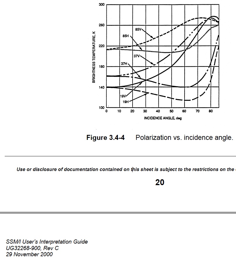
Image of polarization vs. incidence angle.
Image
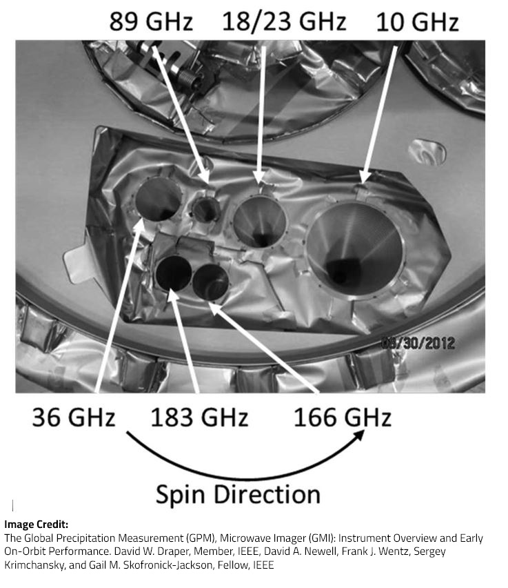
Photograph of the feed horn layout on the GPM Microwave Imager instrument (GMI). Learn more about the GMI.
But, as we've gotten more sophisticated about this stuff, it turns out that having similar EIAs is nice, but in fact we now consider the EIA variations, both between sensors, and for the same sensor due to altitude changes (particularly the TRMM altitude boost to 402.5 km nominal in 2001) and the variations in Earth shape seen by the sensors in ordinary operation.
Precipitation Measurement From Space
Precipitation is measured from space using a combination of active and passive remote-sensing techniques, improving the spatial and temporal coverage of global precipitation observations.
Reliable ground-based precipitation measurements are difficult to obtain because most of the world is covered by water and many countries don’t have precise rain measuring equipment (i.e., rain gauges and radar). Precipitation is also difficult to measure because precipitation systems can be somewhat random and evolve very rapidly. During a storm, precipitation amounts can vary greatly over a very small area and over a short time span. As a result, these systems may fall more- or less-intensely at the location of the ground-based equipment- or it may miss the equipment entirely, introducing error to precipitation estimates.
Fun Fact: Did you know if you gathered all the rain gauges in the world in one place, they would cover an area the size of approximately two basketball courts, or 18,800 square feet (1,740 square meters)? In contrast, satellite observations from space can provide global coverage.
Visible and infrared space-borne sensors can provide precipitation information inferred from cloud-top radiation, and microwave sensors provide direct precipitation measurement based on radiative signatures of precipitating particles. This type of information is not available through ground-based measuring systems. GPM advances space-based measurement even further by combining active and passive sensing capabilities.
GPM
The Global Precipitation Measurement (GPM) is a joint mission co-led by NASA and the Japan Aerospace Exploration Agency (JAXA), and is comprised of an international network of satellites that provide the next-generation global observations of rain and snow. Building upon the success of the Tropical Rainfall Measuring Mission (TRMM), the GPM concept centers on the deployment of a “Core Observatory” satellite carrying an advanced radar / radiometer system to measure precipitation from space and serve as a reference standard to unify precipitation measurements from a constellation of research and operational satellites. Through improved measurements of precipitation globally, the GPM mission is helping to advance our understanding of Earth's water and energy cycle, improve forecasting of extreme events that cause natural hazards and disasters, and extend current capabilities in using accurate and timely information of precipitation to directly benefit society.
Learn more: